Are you struggling to find hidden columns in your Excel spreadsheet? Don’t worry, we’ve got you covered! In this step-by-step guide, we will show you how to easily unhide columns in Excel.
Whether you accidentally hid some columns or received a spreadsheet with hidden information, this guide will help you uncover the hidden data in no time. By following these simple instructions, you’ll be able to navigate to the hidden columns, select them, and access the necessary options to unhide them.
With just a few clicks, you’ll have all the columns visible and ready for editing. So let’s get started and make your Excel experience a whole lot easier!
Key Takeaways
- Unhiding columns in Excel is a simple process that can be done in just a few clicks
- Hidden columns can be uncovered by using the ‘Unhide’ button in the View tab
- The ‘Go To’ feature with Ctrl + G can be used to navigate directly to hidden columns
- The ‘Format’ Tab provides options to customize the appearance of data and unhide columns
Opening Your Excel Spreadsheet
To start uncovering hidden columns in Excel, you’ll need to open your spreadsheet by simply double-clicking on the file. Once you’ve opened the file, you’ll see the Excel interface with your spreadsheet displayed.
Look at the top of the screen for the ribbon, which contains various tabs such as Home, Insert, and View. Click on the View tab to reveal a drop-down menu with different options.
Look for the ‘Hide’ group within the menu and click on the ‘Unhide’ button. This will open a new dialog box where you can select the hidden columns you want to unhide.
Simply check the boxes next to the columns you want to make visible again, and click on the OK button. Your hidden columns will now be uncovered and visible in your Excel spreadsheet.
Navigating to the Hidden Columns
Start by locating the hidden columns in your Excel spreadsheet using the navigation tools provided. To do this, you can either use the scroll bar at the bottom of the screen and drag it to the right or use the arrow keys on your keyboard to move through the columns.
If you know the specific column where the hidden columns are located, you can also use the ‘Go To’ feature. Simply press ‘Ctrl + G’ on your keyboard, enter the column letter and row number of the hidden columns, and click ‘OK’.
This will take you directly to the hidden columns, allowing you to unhide them and make them visible again.
Selecting the Hidden Columns
You can easily reveal the hidden columns in Excel by selecting them. This allows you to uncover valuable information and regain control of your data.
To select the hidden columns, simply click on the column letter to the left of the hidden columns. Hold down the mouse button and drag the cursor to the right until you have selected all the hidden columns. As you select the hidden columns, they will become visible again.
You can also use the keyboard shortcut Ctrl + Spacebar to select the entire column.
Once you have selected the hidden columns, you can perform various actions on them, such as formatting, deleting, or unhiding them permanently.
By selecting the hidden columns, you can efficiently manage and manipulate your data in Excel.
Accessing the “Format” Tab
Once you’ve navigated to the ‘Format’ Tab, you’ll discover a whole range of options to enhance the appearance of your data in Excel. To access the ‘Format’ Tab, simply click on it, and a drop-down menu will appear.
From this menu, you can choose various formatting options such as changing the font, applying borders, and adjusting the cell alignment.
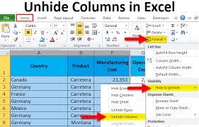
In order to unhide columns, you’ll need to locate the ‘Visibility’ section within the ‘Format’ Tab. Here, you’ll find the ‘Hide & Unhide’ option. Click on it, and another menu will appear. From this menu, select the ‘Unhide Columns’ option, and the hidden columns will reappear in your Excel spreadsheet.
The ‘Format’ Tab provides a convenient and efficient way to unhide columns and customize the appearance of your data.
Choosing the “Hide & Unhide” Option
When selecting the ‘Hide & Unhide’ option from the ‘Format’ Tab in Excel, you gain the power to effortlessly control the visibility of your data. This option allows you to hide or unhide specific columns in your Excel worksheet.
To access this feature, click on the ‘Format’ Tab located at the top of the Excel window. A drop-down menu will appear, and from there, select the ‘Hide & Unhide’ option.
Another drop-down menu will appear, giving you the choice to either hide or unhide columns. If you want to unhide a column, simply select the ‘Unhide Columns’ option.
Once you’ve made your selection, the hidden columns will reappear, making your data visible again.
Unhiding the Hidden Columns
To reveal the hidden columns in Excel, simply select the ‘Unhide Columns’ option from the ‘Hide & Unhide’ menu in the ‘Format’ Tab.
First, click on the ‘Format’ Tab located at the top of the Excel window. Then, locate the ‘Hide & Unhide’ option in the ‘Cells’ group and click on it.
A drop-down menu will appear, and you should select the ‘Unhide Columns’ option. After selecting this option, the hidden columns will be immediately revealed in your Excel spreadsheet.
You can also use the keyboard shortcut ‘Ctrl + Shift + 0’ to unhide columns in Excel. It’s a quick and easy way to bring back any hidden columns and continue working with your data seamlessly.
Frequently Asked Questions
Yes, you can unhide multiple columns at once in Excel. Simply select the range of columns you want to unhide, right-click on any of the selected columns, and choose the “Unhide” option.
If the ‘Format’ tab is not visible in your Excel spreadsheet, you can try enabling it by right-clicking on any visible tab and selecting ‘Customize the Ribbon.’ Then, check the box next to ‘Format’ and click ‘OK.’
Yes, there is a keyboard shortcut to unhide columns in Excel. Simply select the columns you want to unhide and press “Ctrl + Shift + 0” on your keyboard.
Yes, you can unhide columns in a specific range in Excel. Simply select the range of hidden columns, right-click on any column header, and choose “Unhide.” The hidden columns within the range will be unhidden.
To hide columns again in Excel, simply select the columns you want to hide, right-click on them, and choose “Hide” from the drop-down menu. The selected columns will be hidden from view.
Conclusion
In conclusion, un-hiding columns in Excel is a simple process that can be done in just a few steps. By navigating to the hidden columns, accessing the ‘Format’ tab, and choosing the ‘Hide & Unhide’ option, you can easily unhide any hidden columns in your spreadsheet.
Remember, it’s important to know how to unhide columns in Excel to ensure that all the necessary information is visible and easily accessible. So, next time you encounter hidden columns in Excel, follow these steps and unhide them with ease.